Examples🔗

The Python snippets below are included directly from source files under python/examples. Here you can just copy-paste the code to run it locally, or click on the links to open the source files in a new tab.

Optimization with Egor🔗

Unconstrained optimization: Rastrigin 🔗

# =====================================================
# Egobox demo: Minimize Rastrigin with Egor
# =====================================================

import os

import matplotlib
import numpy as np
import egobox as egx
import matplotlib.pyplot as plt

# Comment out the following line to display the plot in a window
matplotlib.use("Agg")


# -----------------------------------------------------
# Define the 2D Rastrigin function
# -----------------------------------------------------
def rastrigin(x: np.ndarray) -> np.ndarray:
    """Rastrigin function."""
    A = 10
    x = np.atleast_2d(x)
    return A * x.shape[1] + np.sum(x**2 - A * np.cos(2 * np.pi * x), axis=1).reshape(
        -1, 1
    )


# -----------------------------------------------------
# Define search space
# -----------------------------------------------------
dim = 2
bounds = [[-5.12, 5.12]] * dim

# -----------------------------------------------------
# Available infill criterion
# -----------------------------------------------------
# Choose one of the following infill strategies: EI, LOG_EI, WB2, WB2S
criterion = egx.InfillStrategy.LOG_EI
print(f"Using infill strategy: {criterion}")

# -----------------------------------------------------
# Initialize optimizer
# -----------------------------------------------------
opt = egx.Egor(bounds, n_doe=20, infill_strategy=criterion)

# -----------------------------------------------------
# Run optimization
# -----------------------------------------------------
optim = opt.minimize(rastrigin, max_iters=80, seed=42)

print("\n===== Optimization Result =====")
print("Best value (y*):", optim.result.y_opt)
print("Best point (x*):", optim.result.x_opt)

# -----------------------------------------------------
# Plot Rastrigin function and sample points
# -----------------------------------------------------
X = np.linspace(bounds[0][0], bounds[0][1], 200)
Y = np.linspace(bounds[1][0], bounds[1][1], 200)
XX, YY = np.meshgrid(X, Y)
XY = np.column_stack([XX.ravel(), YY.ravel()])
ZZ = rastrigin(XY).reshape(XX.shape)

fig = plt.figure(figsize=(7, 6))
plt.contourf(XX, YY, ZZ, levels=50, cmap="viridis")
plt.colorbar(label="Rastrigin value")

# Plot training samples
X_data = np.array(optim.result.x_doe)
plt.scatter(X_data[:, 0], X_data[:, 1], c="red", s=30, label="Sampled points")

plt.scatter(
    optim.result.x_opt[0],
    optim.result.x_opt[1],
    c="white",
    s=100,
    edgecolors="black",
    label="Best point",
)
plt.title("Rastrigin Function - Known Global Minimum = 0 at (0, 0)")
plt.xlabel("x₁")
plt.ylabel("x₂")
plt.legend()
plt.show()

os.makedirs("examples_out", exist_ok=True)
fig.savefig("examples_out/rastrigin.png", dpi=150)

Using infill strategy: InfillStrategy.LOG_EI

===== Optimization Result =====
Best value (y*): [0.00348963]
Best point (x*): [ 0.00415341 -0.00058284]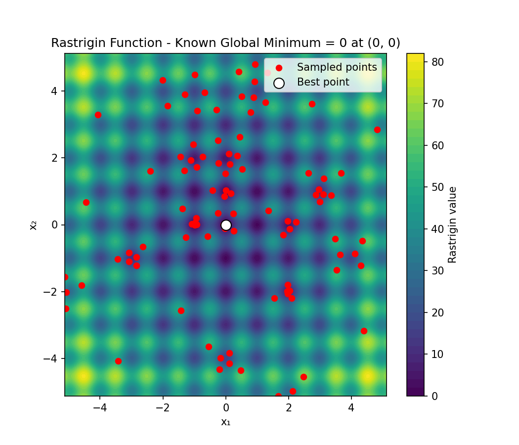

Rastrigin function optimization

Constrained optimization: G24 🔗

import numpy as np
import egobox as egx

# To display optimization information (none by default)
import logging

logging.basicConfig(level=logging.INFO)

xspecs_g24 = [[0.0, 3.0], [0.0, 4.0]]
n_cstr_g24 = 2


# Objective
def G24(point):
    """
    Function g24
    1 global optimum y_opt = -5.5080 at x_opt =(2.3295, 3.1785)
    """
    p = np.atleast_2d(point)
    return -p[:, 0] - p[:, 1]


# Constraints < 0
def G24_c1(point):
    p = np.atleast_2d(point)
    return (
        -2.0 * p[:, 0] ** 4.0
        + 8.0 * p[:, 0] ** 3.0
        - 8.0 * p[:, 0] ** 2.0
        + p[:, 1]
        - 2.0
    )


def G24_c2(point):
    p = np.atleast_2d(point)
    return (
        -4.0 * p[:, 0] ** 4.0
        + 32.0 * p[:, 0] ** 3.0
        - 88.0 * p[:, 0] ** 2.0
        + 96.0 * p[:, 0]
        + p[:, 1]
        - 36.0
    )


# Grouped evaluation
def g24(point):
    p = np.atleast_2d(point)
    return np.array([G24(p), G24_c1(p), G24_c2(p)]).T


# Configure the optimizer. See help(egor) for options
egor = egx.Egor(
    xspecs_g24,
    n_doe=10,
    n_cstr=n_cstr_g24,
    cstr_tol=[1e-3] * n_cstr_g24,
    infill_strategy=egx.InfillStrategy.WB2,
    target=-5.50,  # known reference objective value
)

optim = egor.minimize(g24, max_iters=30)
print(f"Optimization f={optim.result.y_opt} at {optim.result.x_opt}")

Optimization f=[-5.50853583e+00  8.65985077e-04  3.83913510e-04] at [2.32948272 3.17905311]

Surrogate modeling with Gpx🔗

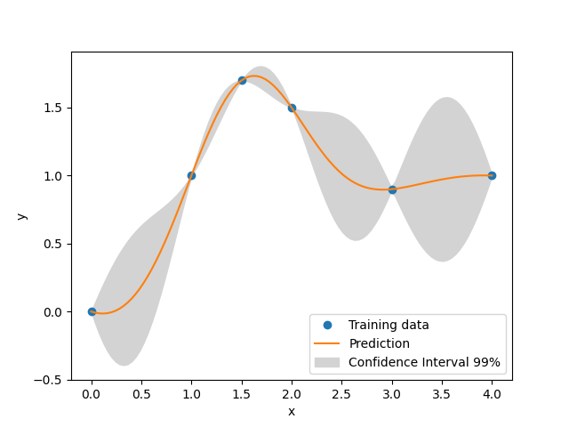
Simple surrogate model: Kriging 🔗

import os

import matplotlib
import numpy as np
import matplotlib.pyplot as plt

# Comment out the following line to display the plot in a window
matplotlib.use("Agg")

import egobox as egx

xt = np.array([[0.0, 1.0, 1.5, 2.0, 3.0, 4.0]]).T
yt = np.array([[0.0, 1.0, 1.7, 1.5, 0.9, 1.0]]).T

gpx = egx.GpMix().fit(xt, yt)

num = 100
x = np.linspace(0.0, 4.0, num).reshape((-1, 1))

y = gpx.predict(x)
# estimated variance
s2 = gpx.predict_var(x)

fig, axs = plt.subplots(1)

# add a plot with variance
axs.plot(xt, yt, "o")
axs.plot(x, y)
axs.fill_between(
    np.ravel(x),
    np.ravel(y - 3 * np.sqrt(s2)),
    np.ravel(y + 3 * np.sqrt(s2)),
    color="lightgrey",
)
axs.set_xlabel("x")
axs.set_ylabel("y")
axs.legend(
    ["Training data", "Prediction", "Confidence Interval 99%"],
    loc="lower right",
)

plt.show()

os.makedirs("examples_out", exist_ok=True)
fig.savefig("examples_out/kriging.png", dpi=150)

Gpx surrogate model

Examples🔗

Optimization with Egor🔗

Unconstrained optimization: Rastrigin🔗

Constrained optimization: G24🔗

Surrogate modeling with Gpx🔗

Simple surrogate model: Kriging🔗

Unconstrained optimization: Rastrigin 🔗

Constrained optimization: G24 🔗

Simple surrogate model: Kriging 🔗